Tag Archives: search engines

A Whirlwind Tour of a Search Engine

Thanks to Krishna Gade and Michael Lopp,  I had an opportunity to speak at Pinterest’s new DiscoverPinterest tech talk series.

I spoke for around 45 minutes, taking the audience on a tour of the world of (mostly) web search — skating across the top of everything from ranking, to infrastructure, to inverted indexing, to query alterations, and more. I had a lot of fun.

Here’s the video:

I also had the chance to listen to four of Pinterest’s engineering leaders discuss their work in browsing, content-based image retrieval, infrastructure, and graph processing and relevance. They’re up to some interesting work — particularly if you’re interested in the intersection of using images, human-curated data, and browsing.

On a social note, it was great to see several of the folks I worked with at Bing. Krishna took a selfie with Yatharth Saraf and I. Those were truly the days — we were in many ways ahead of our time.

Shameless advertisement: if you’d like me to present on search (or anything else) at your organization, please feel free to ask. I have a 30 minute, 1 hour, and whole day tutorial on search engines. I’m also available for consulting and advising!

See you next time.

Measuring Search Relevance

How do you know when you’ve improved the relevance of a search engine? There are many ways to understand this, for example running A/B tests on your website or doing qualitative studies in a lab environment with a few customers. This blog post focuses on using large numbers of human judges to assess search performance.

Relevance Judgment

The process of asking many judges to assess search performance is known as relevance judgment: collecting human judgments on the relevance of search results. The basic task goes like this: you present a judge with a search result, and a search engine query, and you ask the judge to assess how relevant the item is to the query on (say) a four-point scale.

Suppose the query you want to assess is ipod nano 16Gb. Imagine that one of the results is a link to Apple’s page that describes the latest Apple iPod nano 16Gb. A judge might decide that this is a “great result” (which might be, say, our top rating on the four-point scale). They’d then click on a radio button to record their vote and move on to the next task. If the result we showed them was a story about a giraffe, the judge might decide this result is “irrelevant” (say the lowest rating on the four point scale). If it were information about an iPhone, it might be “partially relevant” (say the second-to-lowest), and if it were a review of the latest iPod nano, the judge might say “relevant” (it’s not perfect, but it sure is useful information about an Apple iPod).

The human judgment process itself is subjective, and different people will make different choices. You could argue that a review of the latest iPod nano is a “great result” — maybe you think it’s even better than Apple’s page on the topic. You could also argue that the definitive Apple page isn’t terribly useful in making a buying decision, and you might only rate it as relevant. A judge who knows everything about Apple’s products might make a different decision to someone who’s never owned an digital music player. You get the idea. In practice, judging decisions depend on training, experience, context, knowledge, and quality — it’s an art at best.

There are a few different ways to address subjectivity and get meaningful results. First, you can ask multiple judges to assess the same results to get an average score. Second, you can judge thousands of queries, so that you can compute metrics and be confident statistically that the numbers you see represent true differences in performance between algorithms. Last, you can train your judges carefully, and give them information about what you think relevance means.

Choosing the Task and Running the Judging

You have to decide what queries to judge, how many queries to judge, how many answers to show the judges, and what search engines or algorithms you want to compare. One possible approach to choosing queries is to randomly sample queries from your search engine query logs. You might choose to judge hundreds or thousands of queries. For each query, you might choose to judge the first ten results, and you might choose to compare the first ten results from each of (say) Google, Bing, and DuckDuckGo.

Most search companies do their relevance judgment with crowdsourcing. They put tasks in the public domain, and pay independent people to perform the judgments using services such as CrowdFlower. This does create some problems – some people try to game the system by writing software that randomly answers questions, or they answer fast and erroneously. Search companies have to work constantly on detecting problems, and removing both the poor results and judges from the system. To give you a flavor, one thing search folks do is inject questions where they know what the relevance score should be, and then check that the judges answer most of those correctly (this is known as a ringer test). Another thing folks do is look for judges who consistently answer differently from other judges for the same tasks.

Scoring Relevance Judgments

When you’ve got tens of answers for each query, and you’ve completed judging at least a few hundred queries, you’re ready to compute a metric that allows us to compare algorithms.

An industry favorite is NDCG, Normalized Discounted Cumulative Gain. It sounds complicated, but it’s a common-sense measure. Suppose that on our four-point scale, you give a 0 score for an irrelevant result, 1 for a partially relevant, 2 for relevant, and 3 for perfect. Suppose also that a query is judged by one of the judges, and the first four results that the search engine returns are assessed as relevant, irrelevant, perfect, and relevant by the judge. The cumulative gain after four results is the sum of the scores for each result: 2 + 0 + 3 + 2 = 7. That’s shown in the table below: result position or rank in the first column, the judges score or gain in the second column, and a running total or cumulative gain in the third column.

Rank Judgment (Gain)
Cumulative Gain
1 2 2
2 0 2
3 3 5
4 2 7

Now for the Discounted part in NDCG. Search engine companies know that the first result in the search results is more important than the second, the second more important than the third, and so on. They know this because users click on result one much more than result two, and so on. Moreover, there’s plenty of research that shows users expect search engines to return great results at the top of the page, that they are unlikely to view results low on the page, and that they dislike having to use pagination.

The Discounted part of NDCG adds in a weighting based on position: one simple way to make position one more important than two (and so on) is to sum the score divided by the rank. So, for example, if the third result is ”great”, its contribution is 3 / 3 = 1 (since the score for “great” is 3, and the rank of the result is 3). If “great” were the first result, its contribution would be 3 / 1 = 3. In practice, the score is often divided by the log of the rank, which seems to better match the user perception of relevance. Anyway, for our example and to keep it simple, the Discounted Cumulative Gain (DCG) after four results is 2 / 1 + 0 / 2 + 3 / 3 + 2 / 4 = 3.5. You can see this in the table below: the third column has the discounted gain (the gain divided by the rank), and the fourth column keeps the running total or cumulative gain.

Rank Judgment (Gain)
Discounted Gain Discounted Cumulative Gain (DCG)
1 2 2/1 2
2 0 0/2 2
3 3 3/3 3
4 2 2/4 3.5

The Normalized part in NDCG allows us to compare DCG values between different queries. It’s not fair to compare DCG values across queries because some queries are easier than others: for example, maybe it’s easy to get four perfect results for the query ipod nano, and much harder to get four perfect results for 1968 Porsche 912 targa soft window. If the search engine gets a high score for the easy query, and a poor score for the hard query, it doesn’t mean it’s worse at hard queries – it might just mean the queries have different degrees of difficulties.

Normalization works like this: you figure out what the best possible score is given the results you’ve seen so far. In our previous example, the results scored 2, 0, 3, and 2. The best arrangement of these same results would have been: 3, 2, 2, 0, that is, if the “great” result had been ranked first, followed by the two “relevant” ones, and then the “irrelevant”. This best ranking would have a DCG score of 3 / 1 + 2 / 2 + 2 / 3 + 0 / 4 = 4.67. This is known as the “ideal DCG,” or iDCG.  Our NDCG is the score we got (3.50) divided by the ideal DCG (4.67), or 3.50 / 4.67 = 0.75. Now we can compare scores across queries, since we’re comparing percentages of the best possible arrangements and not the raw scores.

The table below builds out the whole story. You’ve seen the first four columns before. The fifth and sixth columns show what would have happened if the search engine had ordered the results in the perfect order. The seventh and final column shows a running total of the fourth column (the DCG) divided by the sixth column the (ideal or iDCG), and the overall NDCG for our task is shown as 0.75 in bold in the bottom-right corner.

Rank Judgment (Gain)
Discounted Gain Discounted Cumulative Gain (DCG)
Ideal Discounted Gain Ideal Discounted Cumulative Gain (iDCG) Normalized Discounted Cumulative Gain (NDCG)
1 2 2/1 2.0 3/1 3.0 0.67
2 0 0/2 2.0 2/2 4.0 0.5
3 3 3/3 3.0 2/3 4.67 0.64
4 2 2/4 3.5 0/4 4.67 0.75

Comparing Search Systems

Once you’ve computed NDCG values for each query, you can average them across thousands of queries. You can now compare two algorithms or search engines: you take the mean average NDCG values for each system, and check using a statistical test (such as a two sided t-test) whether one algorithm is better than the other, and with what confidence. You might, for example, be able to say with 90% confidence that Google is better than Bing.

As I mentioned at the beginning, this is one important factor you could consider when comparing two algorithms. But there’s more to search engine comparison than comparing NDCG metrics. As I’ve said in previous posts, I’m a huge fan of measuring in many different ways and making decisions with all the data at hand. It takes professional judgment to decide one algorithm is better than another, and that’s part of managing any search engineering effort.

Hope you found this useful, see you next time!

Afterword

I published a first version of this post on eBay’s technical blog in 2010. I owe thanks to Jon Degenhardt for cleaning up a math error, and formatting the tables.

The Cassini Search Engine

Cassini has been in the news lately: Wired.com recently featured a story on Cassini and I was interviewed by eCommerceBytes. Given the interest in the topic, this week’s post is more on the inside Cassini story.

The Beginning

At the end of 2010, we decided that we needed a new search platform. We’ve done great work in improving the existing Voyager search engine, and it had contributed substantially to the turnaround of eBay’s Marketplaces business. But it wasn’t a platform for the future: we needed a new, modern platform to innovate for our customers and business.

We agreed as a team to build Cassini, our new search engine platform. We started Cassini in around October 2010, with a team of a few folks lead by industry veteran Nick Whyte.

Voyager

Our Voyager search engine was built in around 2002. It’s delivered impressively and reliably for over ten years. It’s a good old workhorse. But it isn’t up for what we need today: it was architected before many of the modern advances in how search works, having launched before Microsoft began its search effort and before Google’s current generation of search engine.

We’ve innovated on top of Voyager, and John Donahoe has discussed how our work on search has been important. But it hasn’t been easy and we haven’t been able to do everything we’ve wanted – and our teams want a new platform that allows us to innovate more.

Cassini

Since Voyager was named after the late 1970s space probes, we named our new search engine after the 1996 Cassini probe. It’s a symbolic way of saying it’s still a search engine, but a more modern one.

The Cassini-Huygens probe, the namesake of our Cassini search engine.

The Cassini-Huygens probe, the namesake of our Cassini search engine.

In 2010, we made many fundamental decisions about the architecture and design principles of Cassini. In particular, we decided that:

  • It’d support searching over vastly more text; by default, Voyager lets users search over the title of our items and not the description. We decided that Cassini would allow search over the entire document
  • We’d build a data center automation suite to make deployment of the Cassini software much easier than deploying Voyager; we also built a vision around provisioning machines, fault remediation, and more
  • We decided to support sophisticated, modern approaches to search ranking, including being able to process a query in multiple rounds of ranking (where the first iteration was fast and approximate, and latter rounds were intensive and accurate)

Cassini is a true start-from-scratch rewrite of eBay’s search engine. Because of the unique nature of eBay’s search problem, we couldn’t use an existing solution. We also made a clean break from Voyager – we wanted to build a new, modular, layered solution.

Cassini in 2011

January 2011 marked the real beginning of the project. We’d been working for three or four months as a team of five or so, and we’d sketched out some of the key components. In 2011, we set the project in serious motion – adding more folks to the core team to begin to build key functionality, and embarking on the work needed to automate search. We also began to talk about the project externally.

Cassini in 2012

In 2012, we’d grown the team substantially from the handful of folks who began the project at the end of 2010. We’d also made substantial progress by June – Cassini was being used behind-the-scenes for a couple of minor features, and we’d been demoing it internally.

In the second half of 2012, we began to roll out Cassini for customer-facing scenarios. Our goal was to add value for our customers, but also to harden the system and understand how it performs when it’s operating at scale. This gave us practice in operating the system, and forced us to build many of the pieces that are needed to monitor and operate the system.

The two scenarios that we rolled out Cassini for in 2012 were Completed Search worldwide, and null and low search in North America. Mark Carges talked about this recently at eBay’s 2013 Analysts’ Day.

Completed search is the feature that allows our customers to search listings that have ended, sold or not; it’s a key way that our customers do price research, whether for pricing an item they’re selling or to figure out what to pay when they’re buying. Because Cassini is a more scalable technology, we were able to provide search over 90 days of items rather than the 14 days that Voyager has always offered.

When users get no results from a query (or very few), Voyager offered a very basic solution – no results and a few suggested queries that you might try (this is still what you’ll see on, for example, the Australian site today). Cassini could do much more – it could help us try related queries and search more data to find related matches. After customer testing, we rolled out Cassini in North America, the UK, and Germany to support this scenario – a feature that’s been really well received.

Cassini in May 2013

In January 2013, we began testing Cassini for the default search with around 5% of US customers. As I’ve discussed previously, when we make platform changes, we like to aim for parity for the customers so that it’s a seamless transition. That’s our goal in testing – replace Voyager with a better platform, but offer equivalent results for queries. The testing has been going on with 5% of our US customers almost continuously this year. Parity isn’t easy: it’s a different platform, and our Search Science and Engineering teams have done great work to get us there.

We’ve recently launched Cassini in the US market. If you’re querying on ebay.com, you’re using Cassini. It’s been a smooth launch – our hardening of the platform in 2012, and our extensive testing in 2013 have set us on a good path. Cassini doesn’t yet do anything much different to Voyager: for example, it isn’t by default searching over descriptions yet.

Cassini in 2013 and beyond

We’ll begin working on making Cassini the default search engine in other major markets later in the year. We’re beginning to test it in the UK, and we’ll work on Germany soon too. There’s also a ton of logistics to cover in launching the engine: cassini requires thousands of computers in several data centers.

We’ll also begin to innovate even faster in making search better. Now that we’ve got our new platform, our search science team can begin trying new features and work even faster to deliver better results for our customers. As a team, we’ll blog more about those changes.

We have much more work to do in replacing Voyager. Our users run more than 250+ million queries each day, but many more queries come from internal sources such as our selling tools, on site merchandizing, and email generation tools. We need to add features to Cassini to support those scenarios, and move them over from Voyager.

It’ll be a while before Voyager isn’t needed to support a scenario somewhere in eBay. We’ll then turn Voyager off, celebrate a little, and be entirely powered by Cassini.

See you next week.

Popular Queries

I downloaded the (infamous) AOL query logs a few days back, so I could explore caching in search. Here’s a few things I learnt about popular queries along the way.

Popular queries

The top ten queries in the 2006 AOL query logs are

  1. google
  2. ebay
  3. yahoo
  4. yahoo.com
  5. mapquest
  6. google.com
  7. myspace.com
  8. myspace
  9. http://www.yahoo.com
  10. http://www.google.com

The world’s changed since then: you wouldn’t expect to see a few of those names in the top ten. But what’s probably still true is that the queries are navigational, that is, queries that users pose when they want to go somewhere else on the web. The queries weather and american idol are the only two in the top twenty that aren’t navigational (they’re informational queries).

Misspellings

The misspellings of google are startling. Any spelling you can imagine is in the query logs, and they’re frequent. Here’s a few examples from the top 1,000 queries:

  • googlecom
  • google.
  • http://www.google
  • google.cm
  • googl.com
  • googl
  • goole.com
  • goole
  • goog
  • googel
  • google.co
  • googles
  • goggle.com
  • goggle

This is true of every popular query: a quick glance at ebay (the second-most popular query) finds e-bay, e bay, ebay.com, ebay search, ebay.om, eby, and many more.

And don’t get me started on the different spellings of britney (as in spears): brittanybrittneybritnybritney, …

The good news for users is that most of these misspellings or alternate expressions work just fine at google. That’s the miracle of query rewriting in search.

Single Characters and Other Typing Errors

Single characters queries are surprisingly common. The ten most popular are m (51st most popular query), g (89th), y (115th), a, e, h, w, c, s, and b. Here my theory on m: users are typing <something>.com (which we know is very popular), and at the end they hit enter just before hitting m, and then hit m, and press enter again. Transpositions are pretty common, and m is far-and-away the most popular letter that ends a query. My theory on g and y is they’re the first letters of google and yahoo, and the user hit enter way too early. I don’t have a URL theory on a or e, they are very common letters. On h and w, they’re the beginning of http and www.

There’s many other had-a-problem-with-the interface queries that are popular. Queries such as mhttp, comhttp, .comhttp, and so on are common. What’s happened here is the user has gone back to the search box, partially erased the previous query, typed something new, and hit enter early.

Of the top 1000 queries, 91 begin with www. It’s basically a list of the top sites on the web, that half way through repeats with the initial period replaced with a space (example: http://www.google.com is the 10th most popular query, www google.com is the 123rd most popular query). I wonder if using a www prefix has changed in 6 years? My first theory on this is users don’t get the difference between the search box and the browser address bar — and Google Chrome sure has fixed that problem (make them the one thing). Brilliant, simple innovation. The second theory is that users think they need to put www at the front of queries when they’re navigational — you’ll often hear people talk about that in user experience research sessions.

Caching in Search

Did you know that the vast majority of results from search engines are served from a cache of previously-computed results? Probably only around one third of all queries are actually evaluated using the backend search infrastructure.

Caching provides fast response to most user queries, while allowing search companies to spend much less on hardware, or to devote the resources in their search infrastructure to better computation of results.

Why does caching work in search?

In this post on click curves, I explained that most everything in search follows an inverse power law distribution (a so-called “Zipf curve”). The implication is that a few queries account for the majority of distinct queries, that is, most users are searching for the same things.

AOL memorably released three months of query logs in 2006. They were slammed for doing so and pretty quickly apologized and took down the data. However, it’s a pretty nice data set for our purposes of discussing caching.

The most popular query at AOL in those three months of 2006 was google. Around 0.9% of the queries typed by users were those looking to leave AOL’s search and head over to Google. The second most popular query was ebay at 0.4% of all queries, and the third yahoo at 0.4%. If you sum the frequency of the top ten unique queries, you’ve seen around 3% of all the query volume. Here’s what happens as you inspect more unique queries:

  • If you sum the total frequency of the top 100 queries, you get around 6% of all the user query volume
  • The top 1,000 unique queries are around 11% of the query volume
  • The top 10,000 are around 20% of the volume
  • The top 100,000 are around 34% of the volume
  • The top 1,000,000 are around 58% of the volume

Those points are plotted on a log-log graph below.

Query cache effectiveness for the AOL search query logs. The y-axis is percentage of the total volume of queries that’s cached. The x-axis is the number of unique queries in the cache. Bottom line, storing over a million queries in the cache means you can serve over 60% of user queries from the cache.

We’d expect there’s diminishing returns in caching more queries and their results. As the queries become less frequent, there’s less benefit in caching their results. There’s no benefit in caching a query that occurs once. By the time you’re caching the millionth query from this set, you’re caching queries that occur only 5 times in 3 months. By the way, there are just over 36 million queries in the log, and about 10 million unique queries when they’re normalized (which I didn’t do a very good job of).

The key point to take away is that if we only store only the results for the top 100,000 queries, we can save our search backend from having to evaluate around 34% of all the queries that users pose.

This is a slight exaggeration, since we can’t quite key our search cache on query string alone. Remember that web search users have different language preferences, safe search settings, and so on. All up, the key for our cache probably has around ten parts — but remember than most users likely stick with the defaults, and so the query is the most variable element in the key. I don’t know quite what effect this’d have — but I bet it’s small (say, it reduces the caching effectiveness of the top 100,000 queries from 34% to 32% or so). I expect that the recent Bing and Google pushes into personalization have made caching harder: but I also bet that personalization affects relatively few queries.

Storing Cached Data

The key to the cache is the query and around ten other elements including safe search settings, language preference, market, and so on.

What’s stored in the cache is the results of the query with those settings. For web search, the results includes the list of matching URLs, the snippets, freshness information (more in a moment), and other elements you need to build the page. You might, for example, store the related searches, or the images or news or videos that are associated with queries that show more than web search results.

One of the tricks of caching is knowing when to expire what’s in the cache. You don’t want to keep showing results for a query when the results have actually changed; for example, maybe there’s a new snippet, or a URL has changed, or a new result has entered the top ten results, or there’s some breaking news. Here’s a few factors I thought of that you could use to expire results in the cache:

  • Historical change rate of the results (record how frequently the results change, and use that data to predict when it’ll change in the future)
  • What data is being displayed (if the results contain, for example, news sites, perhaps you expire the cache entry earlier)
  • Change in query frequency (if users suddenly start typing a query much more frequently, that’s a clue that’s something has changed)
  • How long the results have been cached (perhaps you have some time limits that ensure everything is refreshed on a cycle)
  • The load on the search engine (if the search engine is under heavy load, don’t expire the cache as aggressively; if it’s under low load, it’s a good time to refresh the cache)

When you expire a result in the cache, you fall back to the search backend to recompute the results for the query, and then you store those results in the cache.

Bottom line, caching is amazingly effective in search. It’s a super hard problem at eBay, given the dynamic nature of the auction and fixed price formats: items sell, bids change, prices change, and so on. We also blend auctions, fixed price items, and products dynamically based on the results — so even the mix of formats is dynamic. We’re excited about making caching work well at eBay, but we’ve so far not hit anywhere near the heights you’d expect from the analysis of AOL’s web search query logs. I’ll explain this more in the future.

You can learn more about the AOL query logs by downloading this paper from Abdur Chowdhury’s website. Here’s the full citation:

G. Pass, A. Chowdhury, C. Torgeson, “A Picture of Search“, The First
International Conference on Scalable Information Systems, Hong Kong, June,
2006.

I’ll explain some interesting facts about the AOL query logs in a future post.

Ranking at eBay (Part #3)

Over the last two posts on this topic, I’ve explained some of the unique problems of eBay’s search challenge, and how we think about using different factors to build a ranking function. In this post, I’ll tell you more about how we use the factors to rank, how we decide if we’ve improved ranking at eBay, and where we are on the ranking journey.

Hand-tuning a Ranking Function

A ranking function combines different factors to give an overall score that can be used to rank documents from most- to least-relevant to a query. This involves computing each factor using the information that it needs, and then plugging the results into the overall function to combine the factors. Ranking functions are complicated: there’s typically at least three factors in the most simple function, and they’re typically combined by multiplying constants by each of the factors. The output is just a score, which is simply used later to sort the results into rank order (by the way, the scores are typically meaningless across different queries).

If you’ve got two, three, or maybe ten different factors, you can combine them by hand, using a mix of intuition, and experimentation. That’s pretty much what happens in the public domain research. For example, there’s a well-known ranking function Okapi BM25 that brings together three major factors:

  1. Term frequency: How often does a word from the query occur in the document? (the intuition being that a document that contains a query word many times is more relevant than a document that contains it fewer times. For example, if your query is ipod, then a document that mentions ipod ten times is more relevant than one that mentions it once)
  2. Inverse document frequency: How rare is a query word across the whole collection? (the intuition being that a document that contains a rarer word from the query is more relevant than one that contains a more common word. For example, if your query was pink ipod nano, then a document that contains nano is more relevant than a document that contains pink)
  3. Inverse document length: How long is the document? (the intuition being that the longer the document, the more likely it is to contain a query word on the balance of probabilities. Therefore, longer documents need to be slightly penalized or they’ll dominate the results for no good reason)

How are these factors combined in BM25? Pretty much by hand. In the Wikipedia page for Okapi Bm25 the community recommends that the term frequency be weighted slightly higher than the inverse document frequency (a multiplication of 1.2 or 2.0). I’ve heard different recommendations from different people, and it’s pretty much a hand-tuning game to try different approaches and see what works. You’ll often find that research papers talk about what constants they used, and how they selected them; for example, in this 2004 paper of mine, we explain the BM25 variant we use and the constants we chose.

This all works to a certain point: it’s possible to tune factors, and still have a function you can intuitively understand, as long as you don’t have too many factors.

Training Algorithms to Combine Factors

At eBay, we’ve historically done just what I described to build the Best Match function. We created factors, and combined them by hand using intuition, and then used experimentation to see if what we’ve done is better than what’s currently running on the site. That worked for a time, and was key to making the progress we’ve made as a team.

At some point, combining factors by hand becomes very difficult to do — it becomes easier to learn how to combine the factors using algorithms (using what’s broadly known as machine learning). It’s claimed that AltaVista was the first to use algorithmic approaches to combine ranking factors, and that this is now prevalent in industry. It’s certainly true that everyone in the Valley talks about Yahoo!’s use of gradient boosted decision trees in their now-retired search engine, and that Microsoft announced they used machine-based approaches as early as 2005. Google’s approach isn’t known, though I’d guess there’s more hand tuning than in other search engines. Google has said they use more than 200 signals in ranking (I call these factors in this post).

Let me give you an example of how you’d go about using algorithms to combine factors.

First, you need to decide what you’re aiming to achieve, since you want to learn how to combine the factors so that you can achieve a specific goal. There’s lots of choices of what you might optimize for: for example, we might want to deliver relevant results on a per query basis, we might want to maximize clicks on the results per query, we might want to sell more items by dollar value, we might want to sell more items, or we might want to increase the amount of times that a user uses the search engine each month. Of course, there’s many other choices. But this is the important first step — decide what you’re optimizing for.

Second, once you’ve chosen what you want to achieve, you need training data so that your algorithm can learn how to rank. Let’s suppose we’ve decided we want to maximize the number of clicks on results. If we’ve stored (logged or recorded) the interactions of users with our search engine, we have a vast amount of data to extract and use for this task. We go to our data repository and we extract queries and items that were clicked, and queries and items that were not clicked. So, for example, we might extract thousands of sessions where a user ran the query ipod, and the different item identifiers that they did and didn’t click on; it’s important to have both positive and negative training data. We’d do this at a vast scale, we’re likely looking to have hundreds of thousands of data points. (How much data you need depends on how many factors you have, and the algorithm you choose.)

So, now we’ve got examples of what users do and don’t click on a per query basis. Third, it’s time to go an extract the factors that we’re using in ranking. So, we get our hands on all the original data that we need to compute our factors — whether it’s the original items, information about sellers, information about buyers, information from the images, or other behavioral information. Consider an example from earlier: we might want to use term frequency in the item as a factor, so we need to go fetch the original item text, and from that item we’d extract the number of times that each of the query words occurs in the document. We’d do this for every query we’re using in training, and every document that is and isn’t clicked on. For the query ipod, it might have generated a click on this item. We’d inspect this item, count the number of times that ipod occurs, and record the fact that it occurred 44 times. Once we’ve got the factor values for all queries and items, we’re ready to start training our algorithm to combine the factors.

Fourth, we choose an algorithmic approach to learning how to combine the factors. Typical choices might be a support vector machine, decision tree, neural net, or bayesian network. And then we train the algorithm using the training data we’ve created, and give it the target or goal we’re optimizing for. The goal is that the algorithm learns how to separate good examples from bad examples using the factors we’ve provided, and can combine the factors in a way that will lead to relevant documents being ranked ahead of irrelevant examples. In the case we’ve described, we’re aiming for the algorithm to be able to put items that are going to be clicked ahead of items that aren’t going to be clicked, and we’re allowing the algorithm to choose which factors will help it do that and to combine them in way that achieves the goal. Once we’re done training, we’d typically validate that our algorithm works by testing it on some data that we’ve set aside, and then we’re ready to do some serious analysis before testing it on customers.

Fifth, before you launch a new ranking algorithm, you want to know if it’s working sensibly enough for even a small set of customers to see. I’ll explain later how to launch a new approach.

If you’re looking for a simple, graphical way to play around with training using a variety of algorithms, I recommend Orange. It works on Mac OS X.

What about Best Match at eBay?

We launched a machine-learned version of Best Match earlier in 2012. You can learn more about the work we’re doing on machine learning at eBay here.

We now have tens of factors in our ranking function, and it isn’t practical to combine them by hand. And so the 2012 version of Best Match combines its factors by using a machine learned approach. As we add more factors — which we’re always trying to do — we retrain our algorithm, test, iterate, learn, and release new versions. We’re adding more factors because we want to bring more knowledge to the ranking process: the more different, useful data that the ranking algorithm has, the better it will do in separating relevant from irrelevant items.

We don’t talk about what target we’re optimizing for, nor have we explained in detail what factors are used in ranking. We might start sharing the factors soon — in the same way Google does for its ranking function.

Launching a New Ranking Algorithm

Before you launch a new ranking function, you should be sure it’s going to be a likely positive experience for your customers. No function is likely to be entirely better than a previous function — what you’re expecting is that the vast majority of experiences are the same or better, and that only a few scenarios are worse (and, hopefully, not much worse). It’s a little like buying a new car — you usually buy one that’s better than the old one, but there’s usually some compromise you’re making (like, say, not quite the right color, you don’t like the wheels as much, or maybe it doesn’t quite corner as well).

A good place to start in releasing a new function is to use it in the team. We have a side-by-side tool that allows us to see an existing ranking scheme alongside a new approach in a single screen. You run a query, and you see results for both approaches in the same screen. We use this tool to kick the tires of a new approach, and empirically observe whether there’s a benefit for the customers, and what kinds of issues we might see when we release it. I’ve included a simple example from our side by side tool, where you can see a comparison of two ranking for the query yarn, and slightly different results — the team saw that in the experiment on the left we were surfacing a great new result (in green), and on the right in the default control we were surfacing a result that wasn’t price competitive (in red).
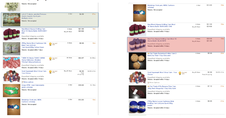
Side by side results for the query yarn. On the left, an experiment, and on the right is the default experience.

If a new approach passes our bar as a team, we’ll then do some human evaluation on a large scale. I explained this in this blog post, but in essence what we do is ask people to judge whether results are relevant or not to queries, and then compute an overall score that tells us how good our new algorithm is compared to the old one. This also allows us to dig into cases where it’s worse, and make sure it’s not significantly worse. We also look at the basic facts about the new approach: for example, for a large set of queries, how different are the results? (with the rationale that we don’t want to dramatically change the customer experience). If we see some quick fixes we can make, we do so.

Once a new algorithm looks good, it’s time to test it on our customers. We typically start very small, trying it out on a tiny fraction of customers, and comparing how those customers use search relative to those who are using the regular algorithms. As we get more confident, we increase the number of customers who are seeing the new approach. And after a few week’s testing, if the new approach is superior to the existing approach, we’ll replace the algorithm entirely. We measure many things about search — and we use all the different facts to make decisions. It’s a complex process, and rarely clear cut — there’s facts that help, but in the end it’s usually a nuanced judgement to release a new function.

Hope you’ve enjoyed this post, the final one in my eBay ranking series. See you again next week, with something new on a new topic!

Ranking at eBay (Part #2)

In part 1 of Ranking at eBay, I explained what makes the eBay search problem different to other online search problems. I also explained why there’s a certain kinship with Twitter, the only other engine that deals with the same kinds of challenges that eBay does. To sum it up, eBay’s search problem is different because our items aren’t around for very long, the information about the items changes very quickly, and we have over 300 million items and the majority are not products like you’d find on major commerce web sites like Walmart or Amazon.

In this post, I explain how we think about using data in the eBay ranking problem. In the next post, I’ll explain how we combine all of that data to compute our Best Match function, and how it’s all coming together in a world where we are rebuilding search at eBay.

Ranking Factors at eBay

Let’s imagine that you and I work together and run the search science team at eBay. Part of our role is to help make sure that the items and products that are returned when a customer runs a query are ordered correctly. Correctly means that the most relevant item to the customer’s information need is in the first position in our search results, the next most relevant is in the second position, and so on.

What does relevant mean? In eBay’s case, you could abstract it to say that the item is great value from a trusted seller, it matches the intent of the query, and it’s something that buyers want to buy. For example, if the customer queries for a polaroid camera, our best result might be a great, used, vintage Polaroid camera in excellent condition. Of course, it’s subjective: you could argue it should be a new generation Polaroid camera, or some other plausible argument. In a general sense, relevance is approximated by computing some measure of statistical similarity — obviously, search engines can’t read a user’s mind, so they compute information to score how similar an item is to a query, and add any other information that’s query independent and can help. (In a future post, I’ll come back and explain how we understand whether we’ve got it right, and work to understand what the underlying intent is behind a query.)

Let’s agree for now that we want to order results from most- to least-relevant to a query, when the user is using our default Best Match sorting feature. So, how do we do that? The key is having information about what we’re ranking: and I’ll argue that the more, different information we have, the better job we can do. Let’s start simply: suppose we only have one data source, the title of the item. I’ve shown below an item, and you can see it’s title at the top, “NICE Older POLAROID 600 Land Camera SUN AUTO FOCUS 660”.

A Polaroid Camera on eBay. Notice the title of the item, "NICE Older POLAROID 600 Land Camera SUN AUTO FOCUS 660"

Let’s think about the factors we can use from the item title to help us order results in a likely relevant way:

  • Does the title contain the query words? The rationale for proposing this factor is pretty simple: if the words are in the title, the item is more relevant than an item that doesn’t contain the words.
  • How frequently are the query words repeated in the title? The rationale is: the more the words are repeated, the more likely that item is to be on the topic of the query, and so the more relevant the item.
  • How rare are each of the query words that match in the title? The rationale is that rarer words across all of the items at eBay are better discriminators between relevant and irrelevant items; in this example, we’d argue that items containing the rarer word polaroid are probably more likely to be relevant than items containing the less rare word camera.
  • How near are the query words to the beginning of the title? The argument is that items with query words near the beginning of the title are likely more relevant than those containing the query words later in the title, with the rationale that the key topic of the item is likely mentioned first or early in the title. Consider two examples to illustrate:  Polaroid land camera 420 1970s issued still in nice shape retro funk, and PX 100 Silver Shade Impossible Project Film for Polaroid SX-70 Camera. (The former example is a camera, the latter example is film for a camera.)

Before I move on, let me just say that these are example factors. I am not sharing that we do or don’t use these factors in ranking at eBay. What I’m illustrating is that you and I can successfully, rationally think about factors we might try in Best Match that might help separate relevant items from irrelevant items. And, overall, when we combine these factors in some way, we should be able to produce a complete ordering of eBay’s results from most- to least-relevant to the query.

So far, I’ve given you narrow examples about text factors from the title. There are many other text factors we could use: factors from the longer item description, category information, text that’s automatically painted onto the item by our algorithms at listing time, and more. If we worked through these methodically, we could together write down factors that we thought might intuitively help us rank items better. At the end of process, I’m guessing we’d have written downs tens of factors for the text alone we have at eBay.

You can see my argument coming together: if you used just one or two of these factors, you might do a good, basic job of ranking items. But if you use more information, you’ll do better. You’ll be able to more effectively discern differences between items, and you’ll do a better job of ranking the items. Net, the more (new, different, and useful) information you have, the better.

What’s key here is that we need different factors, and we need factors that actually do the right thing. There are some simple ways we can test the intuition about a factor before we use it. For example, we could ask a simple question: do users buy more of items that have this factor than those that don’t? In practice, there’s much more sophisticated things we can do to validate a factor before we decide to actually build it into search (and I’ll leave that discussion to another time).

The Factor Buckets

I believe in a five bucket framework of factors to build our eBay Best Match ranking function:

  1. Text factors (discussed above)
  2. Image factors
  3. Seller factors
  4. Buyer factors
  5. Behavioral factors

Pictures or images are an important part of the items and products at eBay. Images are therefore an interesting possible source of ranking factors. For example, we know that users prefer pictures where the background is a single color, that is, where the object of interest is easily distinguished from the background.

The seller is an important part of the buyer’s decision to purchase. You can likely think of many factors that we could include in search: how long have they been selling? How’s their feedback? Do they ship on time? Are they a trusted seller?

Buyer factors is an interesting bucket. If you think about the buyer, there’s many potential factors you might want to explore. Do they always buy fixed price items? What are the categories they buy in? What’s the shoe size they keep on asking for in their queries? Do they buy internationally?

Behavioral factors are also an exciting bucket. Here’s a few examples we could work on: does this item get clicks from buyers for this query? What’s the watch count on the item? How many bids does the auction have? How many sales have their been of this fixed price item, given it’s been shown to users that many times? If you want to dig deeper into this bucket, Mike Mathieson wrote a super blog post on part of our behavioral factor journey.

Where we are on the factors journey

We formed our search science team in late 2009, when Mike Mathieson joined our team. We’ve built the team from Mike to tens of folks in the past couple of years, and we’re on a journey to make search awesome at eBay. Indeed, if you want to join the team — and have an awesome engineering or applied science background, you can always reach out to me.

Right now, we use several text factors in Best Match, we have released a few seller factors and behavioral factors, and we have begun working on image and buyer factors. All up, we have tens of factors in our Best Match ranking function. You might ask: all of these factors seem like they’d be useful, so why haven’t you done more? There’s a few good reasons:

  1. Our current search engine doesn’t make it easy to flexibly combine factors in ranking. (that’s one good reason why we’re rewriting search at eBay.)
  2. It takes engineering time to develop a factor, and make it available at query time for the search ranking process. In many cases, factors are extremely complex engineering projects — for example, imagine how hard it is to process images and extract factors when there’s 10 million new items per day (and most items have more than 1 image), and you’re working hard to get additions to the index complete within 90 seconds. Or imagine how challenging it is to have real-time behavioral factors available in a multi-thousand computer search grid within a few seconds. (If you’ve read Part #1 of this series, you’ll appreciate just how real-time search is at eBay.)
  3. Experimentation takes time. Intuition is the easy part, building the factor, combining it with other factors, testing the new ranking function with users, and iterating and improving takes time. I’ll talk more about experimentation and testing in my next post

In the third and final post in this series, I’ll explain more about how we combine factors and give you some insights into where we are on the search journey at eBay. Thanks for reading: please share this post with your friends and colleagues using the buttons below.

Ranking at eBay (Part #1)

Search ranking is the science of ordering search results from most- to least-relevant in response to user queries. In the case of eBay, the dominant user need is to find a great deal on something they want to purchase. And eBay search’s goal is to do a great job of finding relevant results in response to those customer needs.

eBay is amazingly dynamic. Around 10% of the 300+ million items for sale end each day (sell or end unsold), and a new 10% is listed. A large fraction of items have updates: they get bids, prices change, sellers revise descriptions, buyers watch, buyers offer, buyers ask questions, and so on. We process tens of millions of change events on items in a typical day, that is, our search engine receives that many signals that something important has changed about an item that should be used in the search ranking process. And all that is happening while we process around 250 million queries on a typical day.

In this post, I explain what makes eBay’s search ranking problem unique and complex. I’m aiming here to give you a sense of why we’ve built a custom search engine, and the types of technical search ranking challenges we’re dealing with as we rebuild search at eBay. Next week, I’ll continue this post and offer a few insights into how we’re working on the problem.

What’s different about eBay

Here are a few significantly different facets of eBay’s search problem space:

  1. Under typical load, it takes around 90 seconds from an item being listed by an eBay seller to when it can be found using the search engine. The same is true for any change that affects eBay’s search ranking — for example, if the number of sales of a fixed price multi-quantity item changes, it’s about 90 seconds until that count is updated in our index and can be used in search ranking. Even to an insider, that’s pretty impressive: there’s probably no other search engine that handles inserts, updates, and deletes at the scale and speed that eBay does. (I’ll explain real time index update in detail in a future post, but here’s a paper on the topic if you’d like to know more now.)
  2. In web search, there are many stable signals. Most documents persist and they don’t change very much. The link graph between documents on the web is reasonably stable; for example, my home page will always link to my blog, and my blog posts have links embedded in them that persist and lead to places on the web. All of this means that a web search engine can compute information about documents and their relationships, and use that as a strong signal in ranking. The same isn’t true of an auction item at eBay (which are live for between 1 and 7 days), and it’s less true of a fixed price item (many of which are live for only 30 days) — the link graph isn’t very valuable and static pages aren’t common at eBay
  3. eBay is an ecosystem, and not a search-and-leave search engine. The most important problem that web search engines solve is getting you somewhere else on the web — you run a query, you click on a link and you’re gone. eBay’s different: you run a query, you click on a link, and you’re typically still at eBay and interacting with a product, item, or hub page on eBay. This means that at eBay we know much more than at a web search engine: we know what our users are doing before and after they search, and have a much richer data set to draw from to build search ranking algorithms.
  4. Web search is largely unstructured. It’s mostly about searching blobs of text that form documents, and finding the highest precision matches. eBay certainly has plenty of text in its items and products, but there’s much more structure in the associated information. For example, items are listed in categories, and categories have a hierarchy. We also “paint” information on items as they’re listed in the form of value:attribute pairs; for example, if you list a men’s shirt, we might paint on the item that it is color:green, size:small, and brand:american apparel. We also often know the product that an item is: this is more often the case for listings that are books, DVDs, popular electronics, and motors. Net, eBay search isn’t just about matching text to blobs of text, it’s about matching text or preferences to structured information
  5. Anyone can author a web document, or create a web site. And it’ll happily be crawled by a search engine, perhaps indexed (depends on what they decide to put in their index), and perhaps available to be found. At eBay, sellers create listings (and sometimes products), and everything is always searchable (usually in 90 seconds under typical conditions). And we know much more about our sellers than a web search engine knows about its page authors
  6. We also know a lot about our buyers. A good fraction of the customers that search at eBay are logged in, or have cookies in their browser that identify them. Companies like Google and Microsoft also customize their search for their users when they are logged in (arguably, they do a pretty bad job of it — perhaps a post for another time too). The difference between web search and eBay is that we have information about our buyers’ purchase history, preferred categories, preferred buying formats, preferred sellers, what they’re watching, bidding on, and much more
  7. Almost every item and product has an image, and images play a key role in making purchase decisions (particularly for non-commodity products). We present images in our search results

There are more differences and challenges than these, but my goal here is to give you a taste, not an exhaustive list.

Who has similar problems?

Twitter is probably the closest analog technically to eBay:

  • They make use of changing signals in their ranking and so have to update their search indexes in near real-time too. But it’s not possible to edit a tweet and they don’t yet use clicks in ranking, so that means there’s probably much less updating going on than at eBay
  • Twitter explains that tweet rates go from 2,000 per second to 6000 to 8000 when there is a major event. eBay tends to have signals that change very quickly for a single item as it gets very close to ending (perhaps that’s similar to retweet characteristics). In both cases, signals about individual items are important in ranking those items, and those signals change quickly (whether they’re tweets or eBay items)
  • Twitter is largely an ecosystem like eBay (though many tweets contain links to external web sites)
  • Twitter makes everything searchable like eBay, though they typically truncate the result list and return only the top matches (with a link to see all matches). eBay shows you all the matches by default (you can argue whether or not we should)
  • Twitter doesn’t really have structured data in the sense that eBay does
  • Twitter isn’t as media rich as eBay
  • Twitter probably knows much less about their users’ buying and selling behaviors

(Thanks to Twitter engineering manager Krishna Gade for the links.)

Large commerce search engines (Amazon, Bestbuy, Walmart, and so on) bear similarity too: they are ecosystems, they have structure, they know about their buyers, they have imagery, and they probably search everything. The significant differences are they mostly sell products, and very few unique items, and they have vastly fewer sellers. They are also typically dominated by multi-quantity items (for example, a thousand copies of a book). The implication is there is likely vastly less data to search, relatively almost no index update issues, relatively much less inventory that ends, relatively much less diversity, and likely much fewer changing signals about the things they sell. That makes the search technical challenge vastly different; on the surface it seems simpler than eBay, though there are likely challenges I don’t fully appreciate.

Next week, I’ll continue this post by explaining how we think about ranking at eBay, and explain the framework we use for innovation in search.

Clicks in search

Have you heard of the Pareto principle? The idea that 80% of sales come from 20% of customers, or that the 20% of the richest people control 80% of the world’s wealth.

How about George K. Zipf? The author of the “Human behavior and the principle of least effort” and “The Psycho-Biology of Language” is best-known for “Zipf’s Law“, the observation that the frequency of a word is inversely proportional to the rank of its frequency. Over simplifying a little, the word “the” is about twice as frequent as the word “of”, and then comes “and”, and so on. This also applies to the populations of cities, corporation sizes, and many more natural occurrences.

I’ve spent time understanding and publishing work how Zipf’s work applies in search engines. And the punchline in search is that the Pareto principle and Zipf’s Law are hard at work: the first item in a list gets about twice as many clicks as the second, and so on. There are inverse power law distributions everywhere.

The eBay Search Results Click Curve

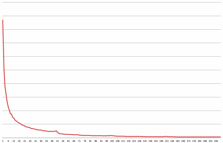
Here’s the eBay search results click curve, averaged over a very large number of queries. The y-axis is the total number of clicks on each result position, and the x-axis is the result position. For example, you can see that the first result in search (the top result, the first item you see when you run a query) gets about eight times as many clicks on average as the fifteenth result. The x-axis is labelled from 1 to 200, which is typically four pages of eBay results since we show 50 results per page by default.

eBay Click Curve. The y-axis is number of clicks per result, and the x-axis is the result position.

As a search guy, I’m not surprised by this curve (more on that topic later). It’s a typical inverse power law distribution (a “Zipf’s Law” distribution). But there are a couple of interesting quirks.

Take a look at the little bump around result position 50 on the x-axis. Why’s that there? What’s happening is that after scrolling for a while through the results, many users scroll to the very bottom of the page. They then inspect the final few results on the page (results 46 to 50), just above the pagination control. Those final few results therefore get a few more clicks than the ones above that the user skipped. Again, this isn’t a surprise to me — you’ll often see little spikes after user scroll points (in web search, you’ll typically see a spike in result 6 or 7 on a 10-result page).

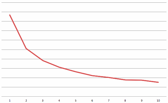
I’ve blown up the first ten positions a little more so that you can see the inverse power law distribution.

Search click curve for the first 10 results in eBay search.

You can see that result 1 gets about 4 times as many clicks as result 10. You can also see that result 2 gets about 5/9ths of the clicks as result 1. This is pretty typical — it’s what you’d expect to see when search is working properly.

Interestingly, even if you randomize the first few results, you’ll still see a click curve that has an inverse power law distribution. Result 1 will almost always get more clicks than result 2, regardless of whether it’s less relevant.

Click Curves Are Everywhere

Here are some other examples of inverse power law distributions that you’ll typically see in search:

  • The query curve. The most popular query is much more popular than the second most popular query, and so on. The top 20% of queries account for at least 80% of the searches. That’s why caching works in search: most search engines serve more than 70% of their results from a cache
  • The document access curve. Because the queries are skew in distribution, and so are the the clicks per result position, it’s probably not surprising that a few documents (or items or objects) are accessed much more frequently than others. As a rule of thumb, you’ll typically find that 80% of the document accesses go to 20% of the documents. Pareto at work.
  • Clicks on related searches. Most search engines show related searches, and there’s a click curve on those that’s an inverse power law distribution
  • Clicks on just about any list: left navigation, pagination controls, ads, and any other list will typically have an inverse power law distribution. That’s why there’s often such a huge price differential between what advertisers will pay in search for the top position versus the second position
  • Words in queries, documents, and ads. Just like Zipf illustrated all those years ago, word frequencies follow an inverse power law distribution. Interestingly, and I explain this in this paper, Zipf’s formal distribution doesn’t hold very well on words drawn from web documents (a thing called Heap’s law does a better job). But the point remains: a few words account for much of the occurrences

What does this all mean? To a search guy, it means that when you see a curve that isn’t an inverse power law distribution, you should worry. There’s probably something wrong — an issue with search relevance, a user experience quirk (like the little bump I explained above), or something else. Expect to see curves that decay rapidly, and worry if you don’t.

See you again next Monday for a new post. If you’re enjoying the posts, please share with your friends by clicking on the little buttons below. Thanks!

Snippets: The unsung heroes of web search

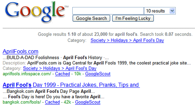
Remember when Google launched into our consciousness? Below you’ll see what you probably saw back in 1999: a clean, simple results page with ten blue links.

Google search results, circa 1999

Google was a marked contrast to the other search engines of the era: AltaVista, Excite, Lycos, Looksmart, Inktomi, Yahoo!, Northern Light, and others.

What was different about Google? Most people talked about three things:

  1. PageRank, the use of the web’s link structure in search ranking. The perception was that Google found more relevant results than its competitors. Here’s the original paper
  2. Its clean page design. It wasn’t a link farm, there was plenty of white space, and an absence of advertising (banner or otherwise) for the first couple of years
  3. Its speed and its collection size. Google felt faster, reported fast search times, claimed a large index (remember when they used to say how many documents they had on the home page?), and showed large result set counts for your queries (result set estimation is a fun game – I should write a blog post about it)

What struck me most was the way Google presented result summaries on the search results page. Google’s result summaries were contextual: they were constructed of fragments of the documents that matched the query, with the query words highlighted. This was a huge step forward from what the others were doing: they were mostly just showing the first hundred or more characters of the document (which often was a mess of HTML, JavaScript, and other rubbish). With Google, you could suddenly tell if the result was relevant to you — and it made Google’s results page look incredibly relevant compared to its competitors.

And that’s what this blog post is about: contextual result summaries in search, snippets.

Snippets

Snippets are the summaries on the search results page. There’s typically ten of them per results page. Take a look at the result below from the Google search engine, it’s one of the ten snippets for the query gold base bobblehead.

A Google Snippet

The snippet is designed to help you make a decision: is this relevant or not to my information need? It helps you decide whether or not to invest a click. It’s important — it’s key to our impression of whether or not a search engine works well. The snippets are the bulk of the results page, they’re displayed below the brand of the search engine, and together they represent what the search engine found in response to your query. If they’re irrelevant, your impression of the search engine is negative; and that’s regardless of whether or not the underlying pages are relevant or not.

The snippet has three basic components:

  1. The title of the web document, usually what’s in the HTML <title> tag. In this case, “Vintage Baseball Memorabilia Bobble Heads Gold Base
  2. A representation of the URL of the web resource, which you can click on to visit the document on the web. In this case, “keymancollectibles.com/bobbleheads/goldbasenod.htm”
  3. (Usually) a query biased summary. One, two, or three fragments extracted from the document that are contextually relevant to the query. In this case, “The Gold base series of Bobbing Heads was the last one issued in the 60’s. They were sold from 1966 through 1971. This series saw the movement of several …”
Some words in the title, URL, and query biased summary are shown in bold. They’re the query words that the user typed (in this case, the query was “gold base bobblehead“) or variants of the query words, such as plurals, synonyms, or acronym expansions or contractions. (My recent post on query rewriting introduces how variants are discovered and used.) The idea here is that highlighting the query terms helps the user identify the likely relevant pieces of the snippet, and quickly make a decision about the relevance of the web resource to their need.

I’m going to come back to discussing query biased summaries, and how the fragments of text are found and ranked. But, before I do, let’s quickly cover what’s been happening in snippets over the past few years.

What’s happening in the world of snippets

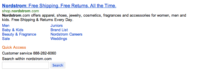
All search engines show quicklinks or deeplinks for navigational queries. Navigational queries are those that are posed by users when they want to visit a specific location on the web, such as Google, Microsoft, or eBay. Take a look at the snippet below from Bing for the query nordstrom. What you can see below the snippet are links that lead to common pages on the nordstrom.com site including “Men”, “Baby & Kids”, and so on; these are what’s known in the industry as quicklinks or deeplinks.  When I was managing the snippets engineering team at Bing, we worked on enhancing snippets for navigational queries to show phone numbers, related sites, and other relevant data. The example for the query nordstrom shows the phone number and a search box for searching only the nordstrom.com site.

Nordstrom navigational query snippet from Bing

At Bing, we also invented customizing snippets for particular sites or classes of sites — for example, below is  a snippet that’s customized for a forum site. You can see that it highlights the number of posts, author, view count, and publication date separately from the query biased summary.

Custom snippet for a forum site from Bing

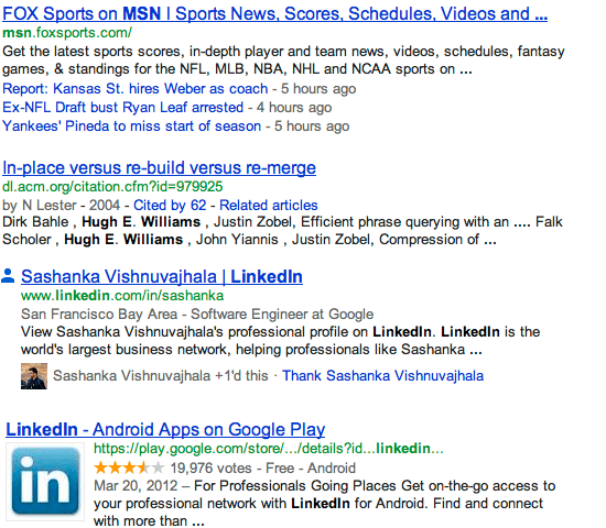
While Bing pioneered it, Google has certainly got in on the game — I’ve included below a few different Google examples for snippets from LinkedIn, Google Play, Google Scholar, and Fox Sports.

Custom Google snippets for LinkedIn, Google Scholar, Google Play, and Fox Sports

What’s all this innovation for? It’s to help users make better decisions about whether or not to click, and to occasionally give extra links to click on. For the Fox Sports snippet, it’s showing the top three headlines from the site — and that’s perhaps what the user wants when they query for Fox Sports (they don’t really want to go to the home page, they want to read a top story). For the Google Play and Scholar snippets, there’s information in the snippet that informs us whether the results is authoritative: has it been cited by other papers many times? Has it been voted on many times? The LinkedIn result is extracting key information and presenting it separately: the city that the person live in and who they work for, and it’s also including some data from Google+.

In my opinion, snippets are becoming too heterogeneous, the search engines are going too far. Users find it hard to switch from processing pictures to reading text, and they’re becoming too intermingled to allow users to quickly scan results pages. The snippets have too many different formats: users have to pause, understand what template they’re looking at, digest the information, and make a decision. The text justification is getting shaky. Life was simpler and faster when snippets were more consistent. I am sure the major search engines would argue that users are making better decisions (for example, I bet they’re seeing on lower mean average times from when the user types a query to when they invest their click). But I think the aesthetics are getting lost, and it’s getting a little too much for most users.

Query-Biased Summaries

Google didn’t invent query-biased summaries, Tassos Tombros and Mark Sanderson invented them in this 1998 paper.

The basic method for producing query-biased summary goes like this:

  1. Process the user’s query using the search index, and get a list of web resources that match (typically ten of them, and typically web [HTML] pages)
  2. For each document that matches:
    1. Find the location of the document in the collection
    2. Seek and read the document into memory
    3. Process the document sequentially and:
      1. Extract all fragments that contain one or more query words (or related terms — you get these from the query rewriting service)
      2. Assign a score to each fragment that approximates its likely relevance to the query
      3. Find the best few fragments based on the best few scores (one, two, or three)
    4. Neaten up the best fragments so they make sense (try and make them begin and end nicely on sentence boundaries or other sensible punctuation)
    5. Stitch the fragments together into one string of text, and save this somewhere
  3. Show the query-biased summaries to the user
I’ve spoken to engineers from the major search companies, and it’s pretty clear that producing snippets is one of the computationally most challenging problems they face. You only execute one query per user request, but you’ve got to produce ten summaries per results page. And unlike the search process, there’s no inverted index structure to help locate the terms in the documents. There are a few tricks that help:
  • Don’t process the entire document. In general, the fragments that are the best summaries are nearer the start of the documents, and so there’s diminishing returns in processing the entirety of large documents. It’s also possible to reorganize the document, by selecting fragments that are very likely to appear in snippets, and putting them together at the start of the document
  • Cache the popular results. Save the query-biased summary after it’s computed, and reuse it when the same query and document pair is requested again
  • Cache documents in memory. It’s been shown that caching just 1% of the documents in memory saves more than 75% of the disk seeks (which turn out to be a major bottleneck)
  • Compress the documents so they’re fast to retrieve from disk. Better still, compress the query words, and compare them directly to the compressed document. This is the subject of a paper I wrote with Dave Hawking, Andrew Turpin, and Yohannes Tsegay a few years ago. We showed that this makes producing snippets around twice as fast as without compression

Most search folks don’t think about the ranking techniques that are used in the snippet generator. The big ranking teams at major search companies focus on matching queries to documents. But the snippet generator does do interesting ranking: its task is to figure out the best fragments in the document that should be shown to the user, from all of the matching fragments in the document. Tombros and Sanderson discuss this briefly: they scored sentences using the square of the number of query words in the sentence divided by the number of query words in the query. Net, the more query words in the fragment, the better. I’d recommend adding a factor that gives more weight to fragments that are closer to the beginning of the document. There are also other things to consider: does the fragment make sense (is it a complete sentence)? Which of the query words are most important, and are those in the fragment? Do the set of fragments we’re showing cover the set of query terms? You could even consider how the set of query-biased summaries give an overall summary of the topic. I’m sure there’s lots of interesting ideas to try here.

Snippets have always fascinated me, and I believe their role in search is critical to users, unsung, and important to building a great search engine.

Hope you enjoyed this post — if you did, please share it with your friends through your favorite social network. There’ll be a new post next Monday…